# Libraries
library(tidyverse)

# Importing eshop_revenues
eshop_revenues <- read_csv("https://raw.githubusercontent.com/DataKortex/Data-Sets/refs/heads/main/eshop_revenues.csv")Simple Linear Regression
Introduction
When we discussed Correlation, we considered how the Pearson correlation coefficient helps us measure the strength and direction of a linear association between two variables. However, with correlation we do not concern ourselves with how one of the variables (the independent variable) predicts the other: we only measure the extend that they “move together” (or oppositely). This—the act of predicting the value of one variable given one or more variables—is where (linear) regression comes in: regression models the relationship between two (or more) variables in a way that explicitly assigns roles: one variable is treated as the dependent variable, which we aim to understand or predict, and the other(s) act as the independent variable(s), which we use to explain the variation in the dependent variable.
In this chapter, we introduce simple linear regression (simple in the sense that only one independent variable is included, as opposed to multiple, and linear in the sense that a linear relationship between the independent and dependent variables is assumed) as the foundation for more complex regression models. We discuss its interpretation, touch upon its mathematical derivation, and—most importantly—we focus on its assumptions and calculation in R. While technical details are essential for building intuition and understanding the foundations of the model, the ultimate goal is to be able to meaningfully interpret regression results as well as to identify model assumptions and limitations.
Understanding the Basics of (Simple Linear) Regression
In its simplest form, regression models the relationship between a dependent and an independent variable as a straight line (hence, linear regression) fitting the data. This line represents the best linear approximation of how the dependent variable changes as the independent variable varies.
To grasp the concept of linear regression, let us focus on the following example: suppose a company sells various products through its online shop. For each product, the company tracks how much it spends on advertising, how many people visit the webpage of the product, the product quality rating, customer satisfaction scores, whether the product is being sold during a holiday season (or not) and whether it is a newly launched item (or not). Finally, the company records the revenue generated from each product (the dependent variable).
In this hypothetical example, we have a sample of product-level data, and our goal is to make statistical inferences for the entire population of products offered by the company. In other words, we aim to understand how different factors influence product revenue, and to estimate these effects in the broader products population, beyond our sample.
We can import this dataset from GitHub using the read_csv() function:
Below is a summary of the dataset (named eshop_revenues):
Ad_Spend(continuous): Advertising spend per product in €Website_visitors(continuous): Number of visitors to the website for the productProduct_Quality_Score(continuous): Quality rating for the productCustomer_Satisfaction(continuous): Customer satisfaction scorePrice(continuous): Product price in €New_Product(dummy 0/1): Whether the product is newRevenue(continuous): Product revenue
As a starting point, in this chapter we will focus on exploring the relationship between Revenue (the dependent variable) and a single independent variable, Ad_Spend.
Generally, a simple linear regression model is of the following form:
\[y = \beta_0 + \beta_1x + u\]
In this equation:
The variable \(y\) is the dependent variable - in our example, product revenue.
The variable \(x\) is the independent variable or predictor - in this simplified example, we will focus on advertising spend.
The variable \(u\) is the error term, representing all other factors that are hypothesized to affect \(y\) but are not included in the model, such as the number of website visitors or customer satisfaction. Note that these variables need not be included in our available dataset - our dataset includes what is made available to us, not necessarily all variables related to our dependent variable.
We use the letter \(u\) for the error term because these omitted factors are unobserved, at least within the scope of the current model. Importantly, we assume that the average value of \(u\) is 0 (Wooldridge, 2022).
The parameters \(\beta_0\) and \(\beta_1\) are, respectively, the coefficients we aim to estimate. These are also referred to as the regression- or model- parameters. Our objective is to find values for these parameters that provide the best linear approximation of the relationship between \(x\) and \(y\) in the population.
The coefficient \(\beta_0\) is called the intercept or constant term. It represents the expected value of \(y\) when \(x = 0\) (assuming the error term \(u\) is also 0, as stated above). In other words, if no advertising spent takes place (i.e., \(x = 0\)), \(y\) is expected to equal \(\beta_0\).
The coefficient \(\beta_1\) is the slope and is a key parameter of interest in simple linear regression. It tells us how much \(y\) is expected to change when \(x\) increases by one unit. Put differently, the slope coefficient \(\hat{\beta}_1\) captures the marginal effect of \(x\) on \(y\).
To understand this more clearly, suppose we increase the value of \(x\) by some amount. The symbol \(\Delta\) (read as “delta” from the respective Greek letter) represents a change in a variable. So, \(\Delta x\) means the change in \(x\), and \(\Delta y\) is the corresponding change in \(y\). Using this notation, the regression equation becomes:
\[\Delta{y} = \Delta{\beta_0} + \beta_1 \Delta{x} + \Delta{u}\]
However, since \(\beta_0\) is a constant, any change in it is zero: \(\Delta{\beta_0} = 0\). Likewise, under the assumption that the expected value of \(u\) is 0 and for all levels of \(x\), we can also claim that \(\Delta{u} = 0\). This leaves us with:
\[\Delta{y} = \beta_1 \Delta{x}\]
This equation means that the change in \(y\) is directly proportional to the change in \(x\), and the proportionality constant is \(\beta_1\).
For example, suppose that \(\beta_1 = 20\). This would imply that for every one-unit increase in \(x\), the expected increase in \(y\) is 20, assuming \(\beta_0\) and \(u\) remain fixed. If \(x\) represents the number of website visitors and \(y\) represents revenue, then gaining one additional visitor would increase revenue by 20 units (whatever the currency or measurement unit is): \[ \Delta{y} = 20 \times \Delta{x} \]An important feature of this model is that the effect of \(x\) on \(y\) is constant: no matter the initial value of \(x\), each additional unit of \(x\) results in the same expected increase in \(y\). This linear relationship is a central assumption of simple linear regression.
The equation
\[y = \beta_0 + \beta_1x + u\]
is known as the Population Regression Function (PRF). It represents the true relationship between \(x\) and \(y\) in the entire population. In this equation, \(\beta_0\) and \(\beta_1\) are the true but unknown parameters that describe this relationship, and \(u\) captures all other influences on \(y\) not included in the model. Because we do not have access to data on the full population, we cannot observe the PRF directly or know the true values of \(\beta_0\) and \(\beta_1\). However, the PRF serves as the theoretical foundation for our analysis—it is the ideal equation we aim to approximate using data from a sample.
When we collect data from a sample and fit a regression line to it, we obtain the Sample Regression Function (SRF). The SRF is written as:
\[\hat{y} = \hat{\beta}_0 + \hat{\beta}_1x\]
Here, \(\hat{\beta}_0\) and \(\hat{\beta}_1\) are estimates of the true population parameters \(\beta_0\) and \(\beta_1\). The hat symbol (^) indicates that these are estimated values. The SRF is our best guess, based on the sample data, of what the PRF looks like. While the SRF may not perfectly match the PRF due to sampling variability and unobserved factors, it provides a useful approximation of the true relationship between \(x\) and \(y\). The goal of regression analysis is to make the SRF as close as possible to the PRF, under the assumptions of the model.
As previously stated, \(u\) represents all the unobserved factors that influence the dependent variable \(y\) but are not included in the model. In our example, such factors could include product reviews, customer loyalty, competition from similar products, or even fluctuations in delivery speed. These variables are not explicitly part of our dataset, but they do affect revenue to some extent.
Since we do not observe these factors, we treat \(u\) as an error term. The typical assumption is that its expected value is 0, meaning that on average, these unobserved influences cancel out. However, we actually assume something even stronger: we assume that the expected value of \(u\), given any value of \(x\), is 0. Formally, this is written as:
\[E(u | x) = E(u) = 0\]
This is a very strong and most often unrealistic assumption. It implies that \(u\) and \(x\) are statistically independent, meaning that no matter what value the independent variable \(x\) takes, the average value of the error term \(u\) remains 0. In this case, for example, we assume that the unobserved factors affecting revenue are not systematically related to advertising spend.
In this context, this would mean that the amount a company spends on advertising is unrelated to any of the omitted variables, such as product quality, brand reputation, or customer satisfaction, that might also influence revenue. This is a very strong and unrealistic assumption because in practice, companies may choose their advertising budget based on such unobserved characteristics. For instance, products with higher quality may receive more advertising, in which case \(x\) and \(u\) would be correlated. This assumption, known as the Zero Conditional Mean, is critically important for estimating the coefficients \(\beta_0\) and \(\beta_1\) accurately, as it forms the foundation for estimating the parameters \(\beta_0\) and \(\beta_1\) using the method of Ordinary Least Squares (OLS) (Wooldridge, 2022).
Visualizing the Linear Regression Line
To grasp the intuition behind OLS, let us first visualize the data. Below is a scatter plot showing the relationship between the independent variable Ad_Spend (on the x-axis) and the dependent variable Revenue (on the y-axis):
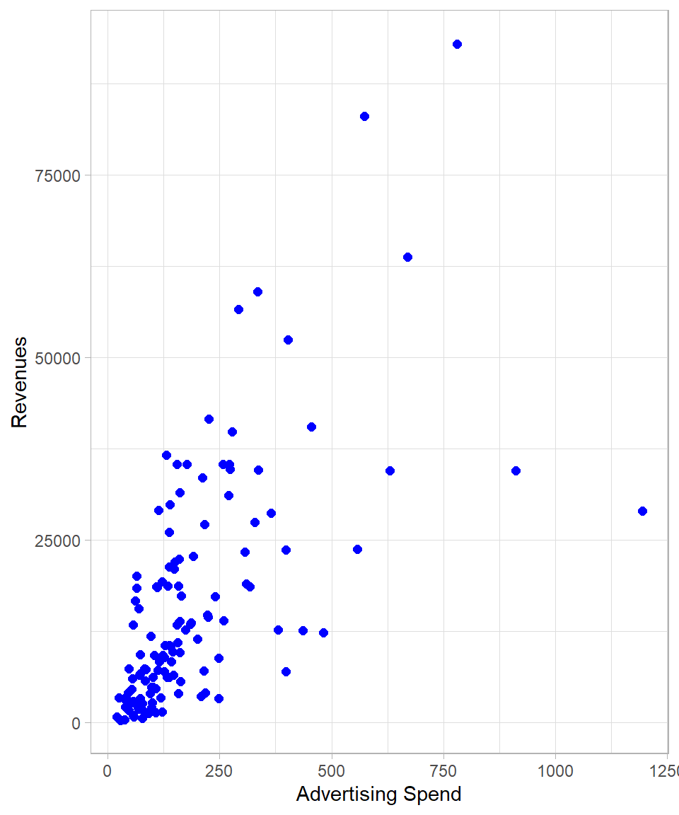
The plot suggests a positive association: in general, the higher the advertising spend, the higher the revenues. Our goal then is to find the best-fitting line that captures this trend, a line that represents the average relationship between advertising spend and revenue and is expressed mathematically through the coefficients \(\beta_0\) and \(\beta_1\). Such a line, and the idea behind OLS, is that it determines the line that minimizes the total squared residuals—that is, the sum of the squared vertical distances between the observed values and the (hypothetical at this moment) fitted line. Indeed, there is one and only one line that satisfies this criterion, and we can find this line by applying the OLS method.
To visualize let us compare two fitted lines:
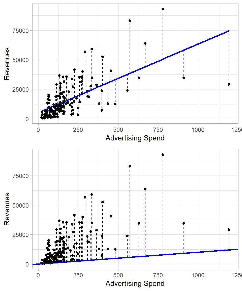
The top plot shows the best-fitting line obtained through OLS. Each dashed vertical segment represents a residual—the difference between the actual value of Revenue and the predicted value, the value of \(y\) that is on the line. These residuals indicate how far the observed data points are from the fitted values.
The bottom plot, by contrast, shows a sub-optimal line. The dashed lines again show residuals, but these are clearly larger in magnitude (when summed) than those in the top plot. This comparison highlights the value of the OLS method: among all possible lines, we choose (calculate) the one that produces the smallest possible sum of squared residuals.
Mathematically, every predicted value on the regression line is given by:
\[\hat{y}_i = \hat{\beta}_0 + \hat{\beta}_1 x_i\]
The difference between the actual value \(y_i\) and the predicted value \(\hat{y}_i\) is the residual, denoted by \(\hat{u}_i\):
\[\hat{u}_i = y_i - \hat{y}_i\]
This is an important concept. In the population model, the term \(u_i\) represented the true error—the influence of all unobserved factors on \(y\). Since we do not observe the population, we cannot know the true errors \(u_i\). However, once we estimate the model using sample data, we can compute the residuals \(\hat{u}_i\), which essentially represent the true errors for our data. If a data point lies exactly on the regression line, then \(y_i = \hat{y}_i\) and the residual is zero.
Deriving Coefficients with OLS
As stated earlier, we derive the coefficients \(\beta_0\) and \(\beta_1\) by starting from the Zero Conditional Mean assumption. Mathematically, this leads to the following two expectations:
\[E(u) = 0\]
\[\text{Cov}(x, u) = E(xu) = 0\]
Here, \(\text{Cov}\) denotes the covariance between the variables \(x\) and \(u\). Covariance is an unstandardized version of the Pearson correlation coefficient. As discussed in Chapter Correlation, the correlation between two variables is calculated by standardizing them—removing the units of measurement—so that the resulting value is bounded between -1 and +1. Covariance, on the other hand, is calculated without standardization, so it retains the units of measurement and is not bounded; it can take any real value.
However, in this context, we are not interested in the specific value of the covariance but in the fact that, under the Zero Conditional Mean assumption, \(x\) and \(u\) are statistically independent. This implies both correlation and covariance are equal to zero.
To estimate the coefficients \(\beta_0\) and \(\beta_1\), we start from the population model:
\[y = \beta_0 + \beta_1x + u\]
Rewriting this, we isolate the error term:
\[u = y - \beta_0 - \beta_1x\]
Taking expectations, and applying the assumption \(E(u) = 0\), we get:
\[E(y - \beta_0 - \beta_1x) = 0\]
\[E(xu) = E[(x \cdot (y - \beta_0 - \beta_1x)] = 0\]
We use these two equations to derive the values of \(\beta_0\) and \(\beta_1\). Since we don’t observe the entire population, we approximate these expectations using the sample data. In practice, this means replacing population expectations with sample averages (after all, these are our best guesses!). This approach gives us two equations, which we then solve to get to the estimated values \(\hat{\beta}_0\) and \(\hat{\beta}_1\):
\[\frac{1}{n} \sum^n_{i = 1}(y_i - \hat{\beta}_0 - \hat{\beta}_1x_i) = 0\]
\[\frac{1}{n} \sum^n_{i = 1}x_i(y_i - \hat{\beta}_0 - \hat{\beta}_1x_i) = 0\]
Let’s start with the first equation:
\[\frac{1}{n} \sum^n_{i = 1}(y_i - \hat{\beta}_0 - \hat{\beta}_1x_i) = 0\]
Distribute the summation:
\[\frac{1}{n} \sum^n_{i = 1}(y_i) = \frac{1}{n} \cdot \sum^n_{i = 1}(\hat{\beta}_0 + \hat{\beta}_1x_i)\]
Since \(\hat{\beta}_0\) and \(\hat{\beta}_1\) are constants, they can be taken out of the summation:
\[\bar{y} = \hat{\beta}_0 + \hat{\beta}_1 \bar{x}\]
Rearranging:
\[\hat{\beta}_0 = \bar{y} - \hat{\beta}_1 \bar{x}\]
This equation shows that once we estimate \(\hat{\beta}_1\), we can directly compute \(\hat{\beta}_0\) using the sample means of \(y\) and \(x\).
Now let’s turn to the second equation:
\[\frac{1}{n} \cdot \sum^n_{i = 1} x_i (y_i - \hat{\beta}_0 - \hat{\beta_1}x_i) = 0\]
Substitute \(\hat{\beta}_0 = \bar{y} - \hat{\beta}_1 \bar{x}\):
\[\sum_{i=1}^{n} x_i \left( y_i - (\bar{y} - \hat{\beta}_1 \bar{x}) - \hat{\beta}_1 x_i \right) = 0\]
Simplify the expression inside the parentheses:
\[y_i - \bar{y} + \hat{\beta}_1 \bar{x} - \hat{\beta}_1 x_i = (y_i - \bar{y}) - \hat{\beta}_1 (x_i - \bar{x})\]
So the equation becomes:
\[\sum_{i=1}^{n} x_i \left[ (y_i - \bar{y}) - \hat{\beta}_1 (x_i - \bar{x}) \right] = 0\]
Now, distribute and simplify the terms:
\[\sum_{i=1}^{n} (x_i - \bar{x})(y_i - \bar{y}) = \hat{\beta}_1 \sum_{i=1}^{n} (x_i - \bar{x})^2\]
Solving for \(\hat{\beta}_1\), we get:
\[\hat{\beta}_1 = \frac{ \sum_{i=1}^{n} (x_i - \bar{x})(y_i - \bar{y}) }{ \sum_{i=1}^{n} (x_i - \bar{x})^2}\]
This is the Ordinary Least Squares estimator for the slope coefficient. Once we compute \(\hat{\beta}_1\), we substitute it back into the equation for the intercept:
\[\hat{\beta}_0 = \bar{y} - \hat{\beta}_1 \bar{x}\]
Putting it all together, the fully estimated regression line becomes:
\[\hat{y}_i = \hat{\beta}_0 + \hat{\beta}_1 x_i\]
This is how the OLS method derives the estimated coefficients. The slope \(\hat{\beta}_1\) tells us how much \(y\) is expected to change for a one-unit increase in \(x\), and the intercept \(\hat{\beta}_0\) tells us the expected value of \(y\) when \(x = 0\).
Calculating in R and Interpreting the Results
To fit a linear regression model in R, we use the lm() function, which stands for “linear model.” This function requires two main inputs: the formula specifying the relationship between the dependent and independent variables, and the data frame that contains these variables.
In our case, we want to regress Revenue (dependent variable) on Ad_Spend (independent variable). In R, the tilde (~) symbol is used to indicate this relationship. The formula Revenue ~ Ad_Spend means: “model Revenue as a function of Ad_Spend:
# Fitting a linear regression model
lm_model <- lm(Revenue ~ Ad_Spend, data = eshop_revenues)

# Printing coefficients
print(lm_model)
Call:
lm(formula = Revenue ~ Ad_Spend, data = eshop_revenues)

Coefficients:
(Intercept)     Ad_Spend
    5110.90        58.17
The output of this command provides the estimates for the coefficients of the regression equation: specifically, the intercept (\(\hat{\beta}_0\)) and the slope (\(\hat{\beta}_1\)). Based on this output, the estimated regression equation is:
\[\widehat{\text{Revenue}}_i = 5110.9 + 58.17 \text{AdSpend}_i\]
Let us review this output in the context of our problem at hand:
\(\hat{\beta}_0 = 5,110.9\): This is the estimated revenue when advertising spend amount is zero. In other words, if the company spent no money on advertising, we would expect revenue to be about €5,110.90. In some contexts, this number may not be very meaningful, especially if \(x = 0\) is outside the range of observed values, but it is still necessary for defining the full regression line.
\(\hat{\beta}_1 = 58.17\): This is the key coefficient, which tells us how much we expect revenue to increase when advertising spend increases by 1 “unit”. In our example, if
Ad_Spendincreases by €1, we expectRevenueto increase by €58.17 (on average). This reflects the marginal effect ofAd_SpendonRevenue.
It is important to emphasize that we are not claiming that every single observation will satisfy:
\[\text{Revenue}_i = 5110.9 + 58.17\text{AdSpend}_i\]
In reality, there will be some variation around this line. What the model gives us is the expected value of Revenue for a given Ad_Spend:
\[E(\text{Revenue}_i | \text{AdSpend}_i) = 5110.9 + 58.17\text{AdSpend}_i\]
This is why we claim that this expectation captures the average relationship across the sample. Each individual observation may be above or below the line, and this difference is just the residual of the corresponding observation.
Once we create an object with the lm() function, we can obtain the fitted values \(\hat{y}\), the residuals \(\hat{u}\) and the coefficients \(\hat{\beta}_0\) and \(\hat{\beta}_1\) using the dollar sign ($) and the corresponding component names. All these values appear as vectors and we can therefore save them in columns in the original data frame for review and additional processing. As fitted values and residuals are returned in the same order as the original observations, we can safely add them back to the data using mutate():
# Obtaining fitted values
lm_model$fitted.values
1 2 3 4 5 6 7 8
11753.518 14353.208 17595.114 23557.706 8394.106 10964.711 12561.522 18107.024
9 10 11 12 13 14 15 16
11784.349 74579.464 24251.694 6739.123 9110.199 14466.643 9281.224 10723.880
17 18 19 20 21 22 23 24
11338.173 7264.995 8838.538 22932.943 13772.656 33107.743 31568.522 28274.844
25 26 27 28 29 30 31 32
13678.418 13063.543 10918.755 14560.881 8393.525 44046.919 8894.964 12887.283
33 34 35 36 37 38 39 40
12406.786 30490.020 15814.480 20099.402 16257.166 14393.929 58118.055 18279.212
41 42 43 44 45 46 47 48
19549.680 22117.376 12150.830 9312.055 9094.493 20871.340 17378.715 6266.770
49 50 51 52 53 54 55 56
10835.570 10958.312 37555.546 13862.240 8543.026 19058.130 15236.254 16812.705
57 58 59 60 61 62 63 64
13142.075 27271.965 14443.374 21322.752 41810.801 11320.139 50470.231 11494.073
65 66 67 68 69 70 71 72
14302.017 9279.479 10828.589 20152.920 14201.962 13329.388 9602.913 10417.897
73 74 75 76 77 78 79 80
7305.715 13065.288 11655.208 7417.986 24668.784 20833.528 18041.872 10085.156
81 82 83 84 85 86 87 88
9288.786 9621.528 12234.598 14116.450 11172.965 17688.770 9557.539 15944.203
89 90 91 92 93 94 95 96
17235.031 12736.037 6603.583 7811.227 7856.600 28581.408 14061.769 7669.288
97 98 99 100 101 102 103 104
7456.380 11952.465 7808.318 28257.974 8323.137 9355.102 15435.201 13127.532
105 106 107 108 109 110 111 112
13110.662 38447.899 9185.822 8410.394 12779.084 24618.757 14491.075 10654.656
113 114 115 116 117 118 119 120
20981.284 23112.693 12467.284 9128.232 13312.518 10007.206 14296.782 14663.263
121 122 123 124 125 126 127 128
17774.282 12172.354 19527.575 13519.609 9862.940 8247.514 26324.931 8440.062
129 130
11424.848 8666.350 # Obtaining residuals
lm_model$residuals 1 2 3 4 5 6
17336.17184 -574.74846 -10491.74361 -4959.03606 -7395.23631 -4723.76081
7 8 9 10 11 12
-2002.27215 -3583.87398 -3427.60912 -45525.45421 3248.15635 -6371.77334
13 14 15 16 17 18
6556.90088 -533.21315 18.37627 1184.16976 -6670.53269 -4005.42491
19 20 21 22 23 24
11245.50240 441.41729 7278.52444 -20797.36315 9014.37827 -21248.17383
25 26 27 28 29 30
-7129.38751 13020.92665 -8147.14521 -8919.38120 5036.78540 19701.93114
31 32 33 34 35 36
9558.19592 5861.07670 -5376.57560 -17809.45964 -2258.17990 15260.64756
37 38 39 40 41 42
6533.89397 8074.79139 -23546.54532 23288.04798 -10694.90050 34497.99359
43 44 45 46 47 48
7142.38958 42.00531 -7045.72278 14516.74999 16220.86487 -5427.06967
49 50 51 52 53 54
-8776.94978 -6069.11193 -13753.20626 8207.07012 -7757.51570 -1753.94019
55 56 57 58 59 60
-2512.88386 -5329.40514 16742.74495 -14564.56486 -4802.57450 18560.39811
61 62 63 64 65 66
-7277.91126 -9893.54949 42498.45936 7013.26733 4438.71257 -2731.29858
67 68 69 70 71 72
-5899.87918 -6137.80034 -3193.42222 -4986.07771 -8939.16286 -9164.53745
73 74 75 76 77 78
-6897.43505 8285.50150 -4465.97810 -5271.07630 9972.92574 10323.18155
79 80 81 82 83 84
-3239.82175 -2767.55570 -5944.96604 -6952.62778 -3020.25757 -666.11992
85 86 87 88 89 90
-1958.49525 9439.21006 -7759.37899 -2252.04264 -13638.76120 23891.38295
91 92 93 94 95 96
-3122.51343 -380.86655 -6155.62042 23902.07166 21386.55142 -5263.39776
97 98 99 100 101 102
-3953.84958 -8477.35514 -3713.25796 -4556.86405 -2283.92692 -2608.59170
103 104 105 106 107 108
20014.30915 -6844.60214 -2503.20237 44656.46088 -6258.40225 -5659.12437
109 110 111 112 113 114
-6568.15406 34413.97335 16993.97476 -6594.19600 13781.33560 -4121.61306
115 116 117 118 119 120
-3473.17410 -7267.38233 -2759.03794 -4271.72572 -10309.81198 2753.25673
121 122 123 124 125 126
-13660.12224 -10656.56392 -16153.20528 -3744.12895 -2490.04006 -3634.51380
127 128 129 130
2373.22933 -5474.72190 7193.93157 8081.01044 # Obtaining estimated coefficients
lm_model$coefficients(Intercept) Ad_Spend
5110.89931 58.17163 # Adding fitted values and residuals to the original data frame
eshop_revenues <- eshop_revenues %>%
mutate(Fitted_Values = lm_model$fitted.values,
Residuals = lm_model$residuals)Units of Measurement
Units of measurement are critically important in regression analysis because they directly affect the interpretation of our coefficients. Suppose Ad_Spend is measured in euro: a one-unit increase then represents a €1 increase.
Now imagine that, instead, we measure Ad_Spend in thousands of euros. In that case, a one-unit increase corresponds to €1,000, not €1. Note how the model adjusts accordingly: the coefficient “shrinks” to 58.17 ÷ 1,000 = 0.05817. The relationship between advertising and revenue has not changed, only the scale has (as the change in sales refers to a change by a thousand euros of advertising spend). This illustrates an important principle: changing the units of a variable will not change the nature of the relationship captured by the regression; instead, the math will rescale the coefficient so that the interpretation remains internally consistent.
The same logic applies to the dependent variable and any other numeric variable in the model. If revenue were measured in euros instead of euros, or in thousands instead of individual units, all coefficients involving revenue would scale accordingly. Converting time from minutes to hours, or distance from kilometers to meters, has the same kind of effect; the regression equation remains valid, but the numerical values of the coefficients adjust to reflect the new units.
This is why being explicit about units is essential. If we misinterpret or ignore them, we might draw incorrect conclusions from the model. Moreover, when comparing results across studies or datasets, it is important to ensure that the units are aligned before comparing coefficients.
In fact, the coefficient \(\beta_1\) depends not only on the strength of the relationship between \(x\) and \(y\), but also on their respective units. This becomes clear when we express \(\beta_1\) using the formula:
\[\beta_1 = r \times \frac{s_y}{s_x}\]
Here, \(r\) is the Pearson correlation between \(x\) and \(y\), and \(s_y\) and =\(s_x\) are the standard deviations of \(y\) and \(x\), respectively. This equation shows that the regression slope is scaled by the ratio of the standard deviations. If we change the units of \(x\) or \(y\), their standard deviations change accordingly — and so does \(\beta_1\). The correlation \(r\), however, remains unaffected by units, as it is constructed to be unit-free.
Statistical Properties
Having derived the OLS estimators, it is instructive to examine several key algebraic properties that follow directly from the equations used to obtain these estimators. These properties help us understand the behavior of residuals and the fit of the regression line.
1. Sum of residuals is 0:
\[\sum^n_{i = 1}u_i = 0\]
This result follows from the first normal equation, which enforces the zero conditional mean in the sample. Because the average of the residuals must match the conditional expectation of the error term (zero), their sum necessarily becomes zero.
In our example, we can confirm this by using the sum() function on the residuals. The resulting number should be very close to 0 (any non-zero outcome is due to the numerical precision used for the calculation):
# Calculating the sum of residuals
sum(lm_model$residuals)
[1] -3.706191e-112. Sample covariance of \(x\) and residuals is zero
\[\sum^n_{i = 1}x_i\hat{u}_i = 0\]
This is equivalent to the second normal equation. It ensures that no linear association remains between the residuals and the explanatory variable. If there were a systematic pattern between \(x\) and the residuals, this would violate the zero conditional mean assumption fundamental to OLS:
# Calculating covariance
sum(lm_model$residuals * eshop_revenues$Ad_Spend)
[1] -2.038723e-083. The regression line always passes through the average values of \(y\) and \(x\)
\[\bar{y} = \hat{\beta}_0 + \hat{\beta}_1 \bar{x}\]
Because we derived \(\hat{\beta}_0 = \bar{y} - \hat{\beta}_1\bar{x}\), the point \((\bar{x},\bar{y})\) lies exactly on the fitted line. Geometrically, this means the average of the observed \(y\) values is the same as the average of the predicted values.
4. Decomposition of Total Variation
Since \(u_i = y_i - \hat{y}_i\), we have the identity:
\[y_i = \hat{y}_i + \hat{u}_i\]
This equation simply says that the actual value of \(y_i\) is equal to the fitted value \(\hat{y}_i\) (the point on the regression line) plus the residual \(\hat{u}_i\) (the vertical distance between the observation and the line). In other words, we can decompose the outcome into what the model explains and what it misses.
Using this idea, we can break down the total variation in the dependent variable \(y\) into two components:
the part explained by the regression model,
and the part left unexplained (the residuals).
This leads to the decomposition of total variation, which separates the total sum of squared deviations into explained and unexplained parts.
- Total Sum of Squares (TSS): Measures the total variation of \(y_i\) around its mean:
\[\text{TSS} = \sum^n_{i = 1} (y_i - \bar{y})^2\]
This is what we would get if we used the mean \(\bar{y}\) to predict every \(y_i\). It’s the benchmark level of variation in the outcome.
- Explained Sum of Squares (ESS): Measures how much of that total variation is captured by the regression model:
\[\text{ESS} = \sum^n_{i = 1} (\hat{y}_i - \bar{y})^2\]
This tells us how much the predicted values \(\hat{y}_i\) deviate from the mean. A large ESS means the model does a good job capturing meaningful variation in \(y\).
- Residual Sum of Squares (RSS): Measures the leftover variation—the part the model fails to explain:
\[\text{RSS} = \sum^n_{i = 1} (y_i - \hat{y}_i)^2\]
Each term \((y_i - \hat{y}_i)^2\) is a squared residual, showing how far the prediction is from the actual value.
These three quantities are related by a fundamental equation:
\[\text{TSS} = \text{ESS} + \text{RSS}\]
This is known as the decomposition of total variation. It tells us that the total variability in \(y\) is exactly split between what is explained by the model (ESS) and what remains in the residuals (RSS).
5. Goodness-of-Fit
The decomposition of total variation is important because it helps us evaluate how well the regression line fits the data. The metric used for this is the coefficient of determination, or \(R^2\), which has the following formula:
\[R^2 = \frac{\text{ESS}}{\text{TSS}} = 1 - \frac{\text{RSS}}{\text{TSS}}\]
This describes the proportion of total variation in \(y\) explained by the model. This is the same \(R^2\), also known as the coefficient of determination. A higher \(R^2\) means a better model, at least in terms of explained variance.
Another way to think about \(R^2\) is that it equals the square of the Pearson correlation coefficient between the observed \(y\) and the fitted values \(\hat{y}_i\):
\[R^2 = [Cor(y, \hat{y})]^2\]
In the following code, we calculate ESS and TSS to find \(R^2\). We also use the cor() function between the fitted values and the actual values to calculate \(R^2\).
# Calculating ESS
ESS <- sum((lm_model$fitted.values - mean(eshop_revenues$Revenue))^2)

# Calculating TSS
TSS <- sum((eshop_revenues$Revenue - mean(eshop_revenues$Revenue))^2)

# Calculating R-squared
ESS / TSS
[1] 0.4030532# Calculating R-squared as squared correlation between Revenue and fitted values
cor(eshop_revenues$Revenue, lm_model$fitted.values)^2[1] 0.4030532As expected, the two methods produce the same \(R^2\) value.
If the regression line passes through all data points perfectly, then \(R^2 = 1\), meaning the model explains all the variance in the dependent variable. On the other hand, the minimum value of \(R^2\) is 0, which means the model does not explain the variation at all. This would occur if the predicted values are always equal to the mean \(\bar{y}\), implying that the independent variable has no explanatory power.
To highlight this point, we create a random variable, Unrelated_Variable, using rnorm() and add it to the dat object with mutate(). Since this variable is unrelated to revenue, we expect the corresponding \(R^2\) to be close to zero.
let’s create a random variable Unrelated_Variable using the rnorm() function to produce values and the mutate() function to connect this new variable to the object dat. Since the new variable is unrelated to the revenue, we expect the corresponding \(R^2\) to be near zero.
# Creating Unrelated_Variable
Unrelated_Variable <- rnorm(nrow(eshop_revenues), mean = 0, sd = 1)

# Connecting Unrelated_Variable to eshop_revenues
eshop_revenues <- eshop_revenues %>%
  mutate(Unrelated_Variable = Unrelated_Variable)

# Fitting linear model with Row_Number as an independent variable
lm_model <- lm(Revenue ~ Unrelated_Variable, data = eshop_revenues)

# Calculating R-squared
cor(eshop_revenues$Revenue, lm_model$fitted.values) ^ 2
[1] 1.488031e-05The resulting \(R^2\) is almost zero, meaning Unrelated_Variable does not explain any variance in Revenue.
Assumptions
When we run a linear regression, we are trying to estimate the line of best fit, i.e., the line that describes the relationship between our dependent variable (e.g. Revenue) and our independent variable (e.g. Ad_Spend) with the least amount of error. But how do we know if the line we estimate is any good?
To trust our regression results, we need to make certain assumptions. These assumptions help us understand when the OLS (Ordinary Least Squares) estimates are reliable and when they might be misleading.
We can break these assumptions into two broad categories:
Assumptions for unbiasedness—to ensure our estimated coefficients, on average, reflect the true values.
Assumptions for efficiency (minimum variance)—to ensure our estimates are as precise as possible.
Let’s go through each category.
Assumption for Unbiasedness
As mentioned above, we want to estimate the coefficients \(\beta_0\) and \(\beta_1\)in a way that the average of our estimates is equal to the true values:
\[E(\hat{\beta_0}) = \beta_0\]
\[E(\hat{\beta_1}) = \beta_1\]
This is what we mean by unbiasedness. If we took many different random samples and estimated the model each time, the average of all those estimates should be equal to the true underlying parameters.
For this to happen, we need the following four assumptions:
1. Linear in Parameters
This assumption states that the true population model must be linear in the parameters—not necessarily linear in the variables. That is, the model should take the form:
\[y_i = \beta_0 + \beta_1 x_i + u\]
This means that the coefficients \(\beta_0\) and \(\beta_1\) are multiplied by known values of \(x_i\) and not by each other, squared, or in any other non-linear form. This assumption is foundational because Ordinary Least Squares (OLS) estimation method relies on solving equations that assume this linearity.
2. Random and Independent Sampling
This assumption means that each observation in our dataset is drawn randomly and independently from the population. This ensures that the observations are representative and not systematically biased in some way. Put differently, knowing the value of one observation gives us no information about the value of any other observation.
3. Sample Variation in the Independent Variable
This means that the independent variable \(x\) must vary in the sample. If all the values of \(x\) are the same, we can’t estimate a slope! There must be some spread in \(x\) so that we can observe how changes in \(x\) are associated with changes in \(y\). This is actually visible in the denominator of the \(\hat{\beta}_1\):
\[\hat{\beta}_1 = \frac{ \sum_{i=1}^{n} (x_i - \bar{x})(y_i - \bar{y}) }{ \sum_{i=1}^{n} (x_i - \bar{x})^2}\]
No sample variation would mean that the denominator would become 0, meaning that we could not estimate \(\hat{\beta}_1\).
4. Zero Conditional Mean
This assumption is the one with which we start the parameter estimation process. It says that the error term has an average of zero, conditional on any value of x:
\[E(u | x) = 0\]
This means that the unobserved factors captured in the error term are not related to the independent variable. If this assumption holds, then \(x\) captures all information needed to explain \(y\) (this could suggest either that all non-informative factors are excluded, or that they cancel out). If it fails, our estimates of \(\beta_1\) will be systematically high or systematically low.
Realistically, this assumption will never hold perfectly in real-world data. There are almost always some unobserved factors that might be correlated with the explanatory variable \(x\). However, the goal in applied regression is to get close enough. Violating the zero conditional mean assumption leads to a serious problem: omitted variable bias, a concept that is discussed in more depth in the next chapter.
Assumptions for efficiency (minimum variance)
The four assumptions above focus on the unbiasedness of our estimates. But unbiasedness only tells us about the average of the estimates, not about how much they vary. However, knowing how far \(\hat{\beta}_1\) and \(\hat{\beta}_0\) can be from the true parameters is critically important because if the estimates vary widely, we might prefer alternative estimators or methods that offer more stability.
Remember, since we estimate \(\hat{\beta}_0\) and \(\hat{\beta}_1\) from a sample, these are random variables. Different samples would give us different estimates. So we care about the variance of these estimates. For this, we need an additional assumption:
5. Homoskedasticity This assumption says that the variance of the error term is constant, regardless of the value of \(x\):
\[Var(u | x) = \sigma^2\]
This looks similar to the zero conditional mean assumption, but now we are focusing on variance instead of the mean. Homoskedasticity means that the spread of the residuals does not depend on \(x\). In simpler terms, the homoskedasticity assumption states that no matter the value of the independent variable, the variance of the errors stays the same.
Let’s see this visually:
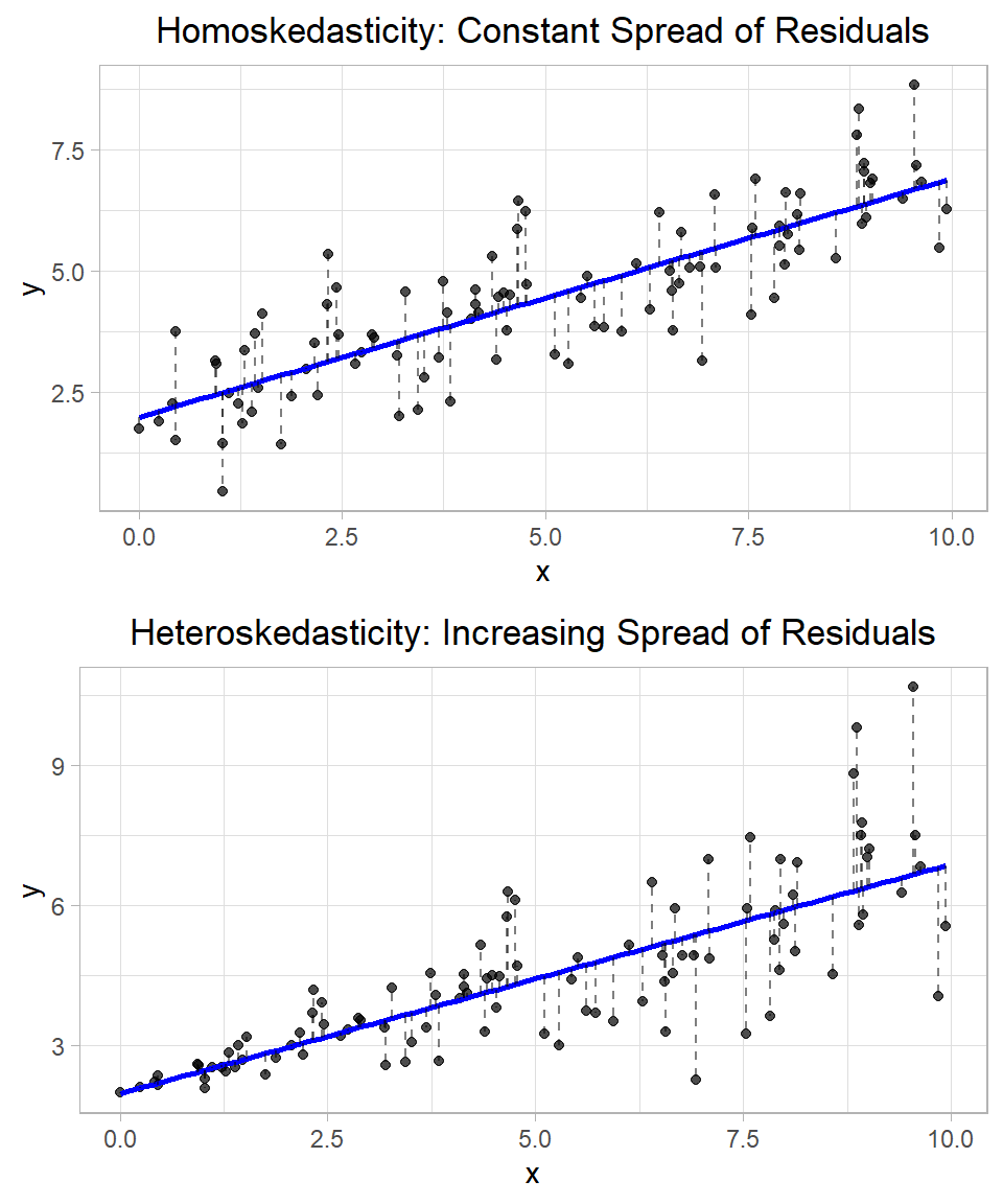
In the top plot, the residuals (shown as dashed red lines) appear to be equally spread out along the fitted regression line, regardless of the value of \(x\). This pattern suggests homoskedasticity—the variance of the error term is constant across all values of the independent variable. In other words, the model’s prediction errors are roughly the same size whether \(x\) is small or large. In the bottom plot, the residuals clearly become larger as \(x\) increases. This pattern indicates heteroskedasticity, which means that the variance of the error term changes with \(x\). In this case, the error terms are not evenly spread—they get wider or narrower depending on the value of the explanatory variable.
In our e-shop example, homoskedasticity would mean that, regardless of how much the company spends on ads, the spread of possible revenues around the regression line stays the same. However, if variance increases with spending—as we saw in the bottom simulated plot—that suggests heteroskedasticity. Perhaps high ad spending sometimes leads to huge returns and sometimes to small returns (depending for example on product qualities?), while low ad spending always leads to predictably low revenue.
The following plot is the scatter plot with Ad_Spend on the x-axis and Revenue on the y-axis. Each point represents an observation in our dataset. We also add the linear regression line, along with a grey shaded area representing the confidence band for the fitted values at each level of the independent variable:
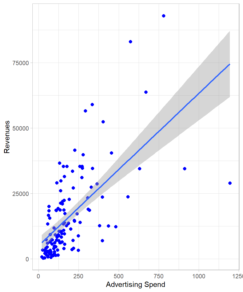
Note how the confidence band around the regression line changes width. This implies that the model detects changing variance, meaning that there is evidence of heteroskedasticity.
The variance of \(\hat{\beta}_1\) reveals some important insights. Firstly, the higher the error variance \(\sigma^2\), the larger the variance of the slope coefficient \(\hat{\beta}_1\). This makes intuitive sense because greater variability in the errors leads to more noise in the data, making it harder to precisely estimate the relationship between \(x\) and \(y\).
On the other hand, the higher the variance of the independent variable \(x\), the lower the variance of \(\hat{\beta}_1\). Intuitively, this occurs because when we have a wider spread or variation in \(x\), we observe more of the underlying relationship between \(x\) and \(y\). Put differently, a larger variance in the independent variable means the data cover a broader range along the regression line, allowing for a more accurate estimation of the slope. This idea is closely related to the concept of sample size: a larger sample size increases the likelihood of capturing the full distribution of \(x\), which in turn improves the precision of our estimate for \(\hat{\beta}_1\). Thus, both lower error variance and greater spread in the independent variable contribute to more reliable and efficient estimates in linear regression.
The \(\sigma^2\) is the variance of the error term \(u\), and that is why \(\sigma^2\) is also called the error variance. Just like \(u\), \(\sigma^2\) refers to the population, not to the sample. And just like the coefficients, we estimate \(\sigma^2\) using the residuals, which represent the errors in our sample.
The variance of the residuals is related to the squared sum of residuals:
\[Var(\hat{u}) = \sum^n_{i = 1} \hat{u}^2_i\]
However, because we work with a sample and not the full population, we must account for degrees of freedom. Since we estimate two parameters (\(\hat{\beta}_0\) and \(\hat{\beta}_1\)) in simple linear regression, we lose two degrees of freedom. Therefore, the degrees of freedom for estimating error variance is:
\[df = n -2\]
where \(n\) is the number of observations.
Therefore, the unbiased estimator of the error variance \(\sigma^2\) is:
\[\hat{\sigma}^2 = \frac{\sum^n_{i =1} {\hat{u}^2_i}}{n - 2}\]
The estimate \(\hat{\sigma}^2\) is called the residual variance and is, on average, equal to the true population variance \(\sigma^2\). In other words:
\[E(\hat{\sigma}^2) = \sigma^2\]
This property makes \(\hat{\sigma}^2\) an unbiased estimator of the population error variance.
Consequently, the standard error of the parameter \(\hat{\beta}_1\) is given by the formula:
\[SE(\hat{\beta}_1) = \sqrt{Var(\hat{\beta}_1)} = \sqrt{\frac{\hat{\sigma}^2}{\sum^n_{i = 1}(x_i - \bar{x})^2}}\]
This standard error reflects the typical amount that \(\hat{\beta}_1\) would vary from sample to sample due to random sampling variation. It plays a central role in constructing confidence intervals and conducting hypothesis tests about \(\beta_1\).
The Gauss-Markov Theorem
If assumptions #1 - #5 hold, then Ordinary Least Squares (OLS) is BLUE—that is, the Best Linear Unbiased Estimator (Wooldridge, 2022). This is also called the Gauss-Markov Theorem, which states:
Under assumptions #1 – #5, the OLS estimator is the best (i.e., has the lowest variance) among all linear and unbiased estimators of the regression coefficients.
To see why this matters, imagine we ignore \(x\) (Ad_Spend) altogether and always predict revenue by its sample average, \(\bar{y}\). That estimator is unbiased—its expectation is the true mean revenue—but it has a variance larger than the linear regression model because it ignores useful information in \(x\) (remember the discussion on variance partitioning, above). OLS, by contrast, incorporates information about the relationship between revenue and Ad_Spend. Under the Gauss–Markov conditions, it not only remains unbiased, but also achieves the smallest possible variance among all unbiased linear estimators (Wooldridge, 2022).
Thus, when Assumptions #1 – #5 are satisfied, OLS is guaranteed to give us the most reliable (i.e. precise) linear estimates of the regression coefficients.
At this point, it is important to note that \(R^2\) is not related with unbiasedness. Theoretically, it is possible that a coefficient is unbiased but the overall \(R^2\) of a linear regression model is very low. Even though a high \(R^2\) would give us more confidence about the the model fit, we should not mix up the concepts.
The Anscombe Plot: A Reminder to Look Beyond the Numbers
A key message in regression analysis is this: we can always fit a line to data—but this does not mean that we should.
To illustrate this, consider the famous Anscombe’s Quartet—a collection of four datasets created by statistician Francis Anscombe in 1973. Each dataset has nearly identical summary statistics: the same mean and variance for both the independent and dependent variables, the same regression line, and even the same \(R^2\) value.
The descriptive statistics are presented below:
# A tibble: 4 × 5
  Dataset   `Average Value X` `Standard Deviation X` `Average Value Y`
  <chr>                 <dbl>                  <dbl>             <dbl>
1 Dataset 1                 9                   3.32              7.50
2 Dataset 2                 9                   3.32              7.50
3 Dataset 3                 9                   3.32              7.5
4 Dataset 4                 9                   3.32              7.50
# ℹ 1 more variable: `Standard Deviation Y` <dbl>
However, when visualized, the datasets look dramatically different:
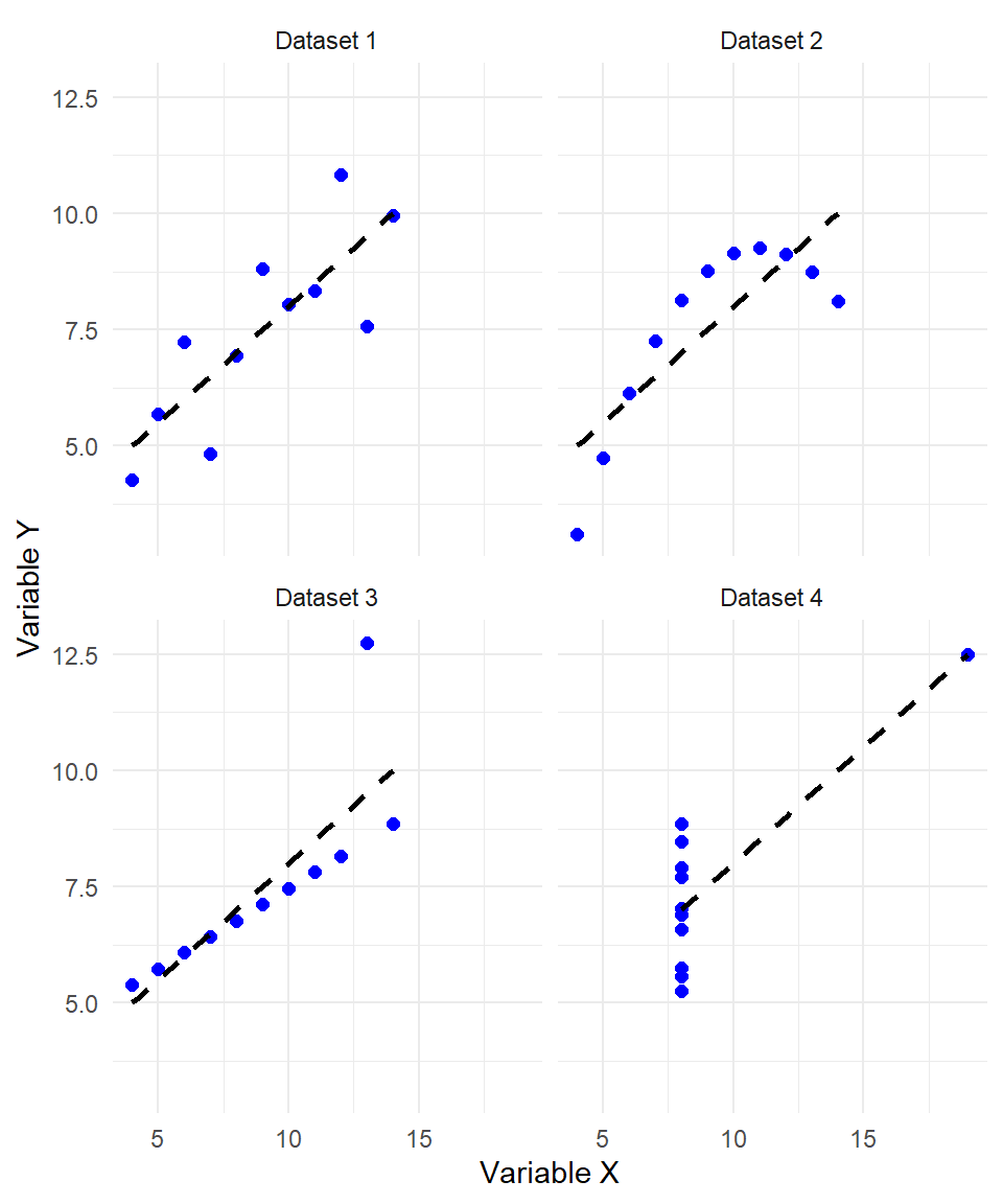
Each plot has the same regression line (shown in red), and each has an \(R^2\) of approximately 0.67. In fact, all datasets have the same descriptive statistical values:
But a closer look reveals:
In Dataset I, the linear relationship appears valid as points are roughly scattered around the regression line.
In Dataset II, the relationship is clearly nonlinear, yet the line still fits because OLS always finds the best-fitting straight line.
In Dataset III, a single outlier drives the regression; removing that one point would completely change the result.
In Dataset IV, all the points lie on a vertical line except for one outlier. Again, the regression line is mathematically valid, but meaningless.
This example shows that summary statistics and \(R^2\) values can be misleading if not complemented with visual inspection and contextual understanding. While Dataset I likely satisfies the assumptions for unbiased and efficient estimation, the other datasets violate key assumptions such as linearity, constant variance, and sufficient variation in the independent variable. As a result, their slope estimates may be biased or inefficient. For example, in Dataset IV, removing the single outlier would leave no variation in the independent variable, violating the assumption required for regression to be meaningful at all.
Therefore, the Anscombe plot reminds us of several critical points:
OLS will always produce a line, even when the data clearly violate the assumptions behind regression such as linearity, constant variance, and lack of extreme outliers.
A high \(R^2\) does not guarantee that the model is appropriate or meaningful. Therefore, visualizing the data is essential. Before interpreting coefficients or evaluating model fit, it’s important to actually look at the data.
Understanding the data-generating process is critical. What the variables represent, what relationships make sense, and whether the assumptions of regression are reasonable, are all key parts of the modeling process.
Assumptions matter: We assume that residuals are centered around zero (unbiasedness), that errors are homoskedastic, and that the model captures a linear relationship. These assumptions are not just technical details — they define when and how regression results can be trusted.
In short: Just because we can fit a line, doesn’t mean the line tells us something useful. Statistics is not only about numbers—it’s also about thinking critically and combining quantitative tools with domain knowledge and visual insight.
Notes Regarding Language
Before we wrap up this chapter, it is important to emphasize some subtle yet essential points about the language used in regression analysis.
First, Ordinary Least Squares (OLS) is a method, not a model. The model refers to the theoretical relationship we assume between the dependent and independent variables, such as a linear function involving \(x\) and an error term \(u\). OLS is the method we use to estimate the parameters of that model from the data.
Second, when we say an estimator is unbiased, we mean that its expected value equals the true parameter across repeated samples. This does not imply that the estimate from a single dataset is equal to the true value. For example, \(\hat{\beta}_1 = 2.7\) might not equal \(\beta_1\), but as long as \(E(\hat{\beta}_1) = \beta_1\), the estimator is unbiased.
Last but not least, when we say independent variables “explain” or “predict” the dependent variable, we are referring to a statistical relationship—not a causal one. Unless we have carefully designed the model for causal inference, we cannot claim that one variable causes another; we can only say they are associated.
A Brief History of Linear Regression: Gauss, Galton, and the Birth of a Statistical Tool
The idea behind linear regression has deep historical roots, with contributions from both Carl Friedrich Gauss and Francis Galton, two figures who worked on regression independently, each with their own different reasons for doing so (Gauss, 1809; Galton, 1886; Pearl & Mackenzie, 2018).
The mathematical foundation of linear regression goes back to the early 19th century, when Carl Friedrich Gauss introduced the method of least squares. He used it around 1795 to predict the orbits of celestial bodies—especially the asteroid Ceres—based on scattered astronomical observations (Gauss, 1809).
Gauss’s idea was simple but powerful: choose the line (or curve) that minimizes the sum of squared differences between the observed values and the values predicted by the model. This is exactly what we now call Ordinary Least Squares (OLS) (Legendre, 1805).
Although another mathematician, Adrien-Marie Legendre published the method in 1805, Gauss claimed to have used it earlier and provided a probabilistic justification by 1809 (Gauss, 1809). His motivation was astronomical prediction, not the analysis of human traits or social data.
He is also the reason why the normal distribution is often called the Gaussian distribution, since he was one of the first to describe its properties and apply it in the context of measurement errors and statistical inference—concepts that are central to regression analysis (Pearl & Mackenzie, 2018).
Francis Galton, a 19th-century British polymath and cousin of Charles Darwin, gave the concept of regression its name. In the late 1800s, Galton studied heredity in human height, trying to understand how traits are passed from parents to children (Galton, 1886; Pearl & Mackenzie, 2018).
In his famous study, Galton found that:
Tall fathers tend to have tall sons, but
The sons were, on average, closer to the population mean than their parents.
This phenomenon—“regression toward mediocrity” as he called it—was one of the first empirical demonstrations of what we now call regression to the mean (Galton, 1886). Galton plotted father and son heights and noticed a linear pattern, which he quantified using what we would now recognize as a simple linear regression. In other words, he used the height of fathers as the independent variable and the height of sons as the dependent variable, fitting a line to predict sons’ heights based on their fathers’ heights.
While Galton didn’t develop the mathematics of least squares, he played an important role in introducing regression as a concept in the context of human traits. His work was later formalized and extended by Karl Pearson, who developed the correlation coefficient and more of the modern regression framework (Pearson, 1896).
Recap
In this chapter, we explored the foundation of simple linear regression, focusing on how we can model the relationship between a single independent variable and a dependent variable using a straight line. We examined the components of the regression equation, interpreted the slope and intercept, and understood how the model’s fitted values and residuals arise from observed data. We also discussed the Ordinary Least Squares (OLS) method for estimating the model parameters, emphasizing its desirable property of unbiasedness under certain key assumptions.
We further investigated the variance of the slope estimator, showing how it depends both on the error variance and the spread of the independent variable. We stressed the importance of understanding assumptions like homoskedasticity, independence, and variability in the data. Through graphical examples such as Anscombe’s Quartet, we saw that even when numerical summaries such as \(R^2\) are identical, the reliability of the regression can vary dramatically.
In the next chapter, we will move beyond the simple case and introduce multiple linear regression, where we include more than one independent variable.